1. Types of data
How to describe and summarize data
4.56/5 (9)
Qualitative data
Qualitative data can either be measured on a nominal scale or an ordinal scale. Some qualitative variables such as disease diagnosis have no inherent order – they are classified by name on a nominal scale.
Other qualitative variables such as the level of anxiety has a natural order and can therefore be classified on an ordinal scale, for example, no anxiety, mild anxiety, moderate anxiety and severe anxiety.
Some qualitative information can both be grouped on a nominal scale and on an ordinal scale. For example, pain can be classified by type on a nominal scale (stinging, burning, stabbing, pressing, etc.) and in regard to intensity on an ordinal scale (no pain, mild pain, moderate pain and severe pain).
For any variable the classes should be exhaustive, i.e. any observation should be placed in one of the defined classes. In addition, the classes should be mutually exclusive, i.e. no observation should be classified simultaneously in more than one class.
The latter requirement may be difficult to achieve in practice for qualitative variables (e.g. see the WHO disease classification).
–
Proportion
Qualitative data are summarized by their frequency or proportion P being the number with the characteristic in question divided by the number of individuals in the sample. If in a sample of 80 only 25 have pain, then the proportion P with pain is 25/80 = 0.31 or 31%.
–
Quantitative data
Quantitative variables are always ordinal, i.e. they always have a built-in sequence, as they can be arranged according to value.
The distance between the steps on the scale need not be constant. For example, the distance from 5 mm to 10 mm of pain on a visual analog scale is not necessarily assumed to represent the same increase in pain intensity as the distance from 10 mm to 15 mm on the scale.
For many quantitative variables, however, a given interval represents the same change in the whole range of the scale. Such variables are measured on a ratio-interval scale. Quantitative variables usually have a natural zero, but it does not always apply (e.g. temperature, where zero is different depending on whether you measure in Celsius or Fahrenheit).
A variable may be discrete or continuous. Discrete variables can only assume a limited number of values. Many variables can only assume two values (e.g. gender, living /dead, yes /no) – they are called binomial or dichotomous. Continuous variables can assume any value within a range, but many may only be positive (as height, weight, bilirubin concentration in the blood, blood pressure).
–
Describing the distribution of quantitative data – the histogram
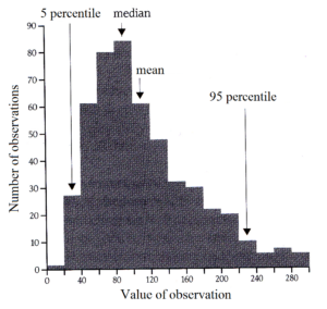
 The distribution of quantitative data in a population or a sample can be illustrated in a histogram. It shows the data in intervals according to their value and the number in each interval.
The value of the variable is plotted in intervals of equal size on the x-axis, while the y-axis gives the number (or percentage) of observations in each interval. The distribution of the data can be summarized by several different numbers.
The two most important elements in the description are: measures of the centre of the distribution (the central tendency) and measures of the scatter of observations around the middle.
–
Measures of the center of the distribution (the central tendency)
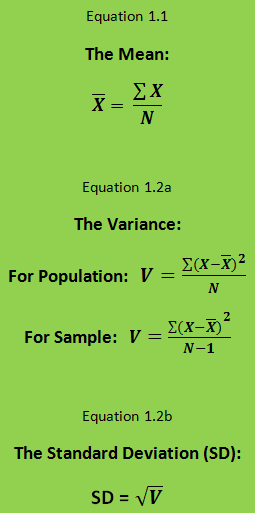
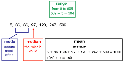
The mean or average is defined as the sum of the observations divided by their number as in equation 1.1.
The mean is best suited for symmetric distributions. For a skewed distribution the mean is pulled disproportionately toward the long “tail”.
The median is defined as the middle value, i.e. half of the observations are below and half are above the median.
The mode is the most frequent value.
Determination of the median implies that the values are sorted in order of size. The median is affected to a lesser degree than the mean of the long tail of skewed distributions.
–
Measures of the scatter of observations around the middle
The Standard Deviation (SD). This is the square root of the variance (V), see equation 1.2b. The variance (V) for a population is the sum of the squared deviations of the observations from the mean divided by the number of observations. For a sample the denominator should be the number of observations minus one. See equation 1.2a. This is a way of compensating for studying only a part of the population (the sample) and not the total population.
The standard deviation in percent of the mean is called the coefficient of variation.
The mean and standard deviation are most useful for symmetric distributions – especially for the normal distribution.
 The range is the difference between the largest and smallest observation: maximum value minus minimum value. Sometimes only the minimum and maximum values are given.
This measure of the variation in the data is always useful and informative, no matter the shape of the distribution.
Quartiles. The three quartiles divide the sorted data in 4 equal parts each representing a quarter of the data.
The interquartile range is the middle 50% of the range i.e. upper quartile (Q3) minus the lower quartile (Q1).
Percentiles. Any distribution of data can be described in more detail using percentiles. Identification of the percentiles requires that the observations are sorted.
The 0th percentile corresponds to the smallest observation, the 50th percentile corresponds to the median and the 100th percentile corresponds to the highest observation.
In general, the nth percentile is the upper limit of the smallest n% of the observations.
An acceptable summary description of the variation could be the difference between the 95th – and 5th percentile, or between the 90th – and the 10th percentile.
Compute online
Here is a link to a page, where you can calculate online the parameters described plus some extra. Just copy and paste your data e.g. from a spreadsheet program.


