6. Statistical tests
4.5/5 (6)
Parametric tests
Many statistical tests are parametric, i.e. they require a known distribution, usually a normal distribution. The assumption of normal distribution applies to the parameters you want to compare, for example the mean of the effect variable in the groups.
Mean values will be approximately normally distributed, either if the variable itself is normally distributed or if the number of observations in each group is so large that the mean can be assumed to be normally distributed, regardless of the underlying distribution of the data values.
Before using parametric tests, one should consider whether the effect variable can be assumed to be normally distributed, or, as will be seen, if the variable if necessary can be made to be normally distributed by a suitable transformation.
Variables which an organism keeps regulated within narrow limits (e.g. blood pressure) will usually be distributed symmetrically around the optimum value, and the distribution is usually so close to the normal, that it does not cause problems in statistical analysis, which assumes a normal distribution.
Logarithmic transformation of variable
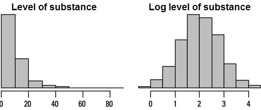
For variables that an organism attempts to keep below a certain level, the distribution tends to be skewed with most of the values in the low range and a longer tail of higher values.
Experience shows that this type of variable often will follow a normal distribution rather closely after a logarithmic transformation. An example is the concentration of creatinine in the blood. Creatinine is a waste product, which is removed from the organism by the kidneys.
The effect of the kidneys on the variable is proportional to the level of creatinine in the blood. By taking the logarithm of the creatinine concentration, the distribution of the values becomes close to the normal distribution.
Test for normality
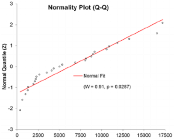
Before using parametric tests, one should always check the assumption of normal distribution using a frequency plot, which gives a visual presentation of the distribution of the data. Then you can see whether the distribution is bell-shaped and reasonably symmetrical, and you will easily be able to detect any outliers.
It can be difficult to assess the tails of the distribution. It may be helpful to look at the cumulative frequency distribution, which – in a diagram with the Normal Deviate Z on the y-axis – is shown as a straight line if the distribution is normal.
You can use Shapiro-Wilk’s test to determine if the distribution can be considered normal.
Compute Online
Here are two links to online calculators where you can perform the Shapiro-Wilk test: Link 1, Link 2.
Non-parametric tests
If the data is not normally distributed, it will in the analysis of large data sets often pay to find out how the distribution deviates from the normal distribution, and then by appropriate transformation of the variable ensure that distribution is appropriate normal. When analyzing small populations will often lead us too far to analyze any deviations from the normal distribution, and you can instead get around the problem by using a test that does not require a normal distribution
Although nonparametric tests usually requires certain assumptions about the distribution are met, they are also called distribution-free tests because the conditions are less restrictive than the assumption of normal distribution. The Mann-Whitney test, referred to below, is an example of a non-parametric test, whereas the t-test is parametric.
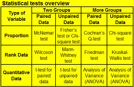
 The following points are important to choose the appropriate statistical test:
- Data paired or unpaired?
- Number of groups to compare: two or more?
- Type of effect variable: proportion, rank data or quantitative data?
A. Tests for Proportions
A1. Comparison of Two Paired Proportions: McNemar’s test
McNemar’s test is used on dichotomous data in matched pairs of subjects. The test is applied to a 2×2 contingency table, which tabulates the outcomes of two tests on a sample of n subjects.
Compute Online
Here you can compute McNemar’s test online. The link does also provide an exact binomial test.
–
–
A2. Comparison of Two Independent Proportions: Fisher’s exact test or the Chi-square (χ²) test
These tests analyze a dichotomous variable in two independent groups. The tests are applied to a 2×2 contingency table, which tabulates the outcomes of the variable (e.g. ±pain) in two independent groups (e.g. males and females) to be compared. Fisher’s exact test is exact even for small samples, while the Chi-square test gives an approximation, which is good for large but not for small samples. The principle in the Chi-square test is to compare the observed numbers in the 2×2 table with the numbers expected if the proportions were the same in the two groups.
Compute Online
In this link you can compute both Fisher’s exact test and the Chi-square test.
Here you can calculate the the Confidence Interval for the difference between two independent proportions.
A3. Comparison of More Paired Proportions: Cochran’s Q-test
Cochran’s Q-test analyses a binary response (success/failure or 1/0) in three or more matched groups (groups of the same size). The test assesses whether the proportion of successes is the same between groups. This test can be regarded as an extension of McNemar’s test for more than two groups.
Compute Online
In this link, you can compute Cochran’s Q-test.
–
–
A4. Comparison of Categorical Data in More Groups: the Chi-square (χ²) test
The Chi-square (χ²) test for more categories and groups is a test of independence between the groups. The data can be displayed in an R×C contingency table, where R stands for the number of categories (organized in Rows) and C stands for the number of groups (organized in Columns). The chi-square test of independence can be used to examine the relationship between the groups and categories. The null hypothesis is that there is no such relationship. If the null hypothesis is rejected the implication would be that the categories differ between the groups.
Compute Online
In this link you can calculate the Chi-square (χ²) test for a R×C contingency table.
B. Non-parametric Tests using Rank Data
B1. Comparison of Two Paired Sets of Rank Data: The Wilcoxon Signed Rank Test.
The Wilcoxon signed-rank test is a non-parametric paired difference test used to compare two related samples, matched samples, or repeated measurements on a single sample to assess whether their rank sums differ. It can be used as an alternative to the paired Student’s t-test, when the data cannot be assumed to be normally distributed.
Compute Online
Using this link you can perform the Wilcoxon signed-rank test online. The confidence interval of the result is also provided. You should use the original data since the program will calculate the ranks from the data. Remember to select the Wilcoxon signed-rank test in the link.
–
–
B2. Comparison of Two Independent Sets of Rank Data: The Mann-Whitney Test
The Mann–Whitney test is a non-parametric test used to compare quantitative or rank data in two unrelated samples. It can replace the unpaired Student’s t-test, when the assumption of normal distribution is not fulfilled.
Compute Online
Using this link you can perform the Mann-Whitney test online. The confidence interval of the result is also provided. You should use the original data since the program will calculate the ranks from the data. Remember to select the Mann-Whitney test in the link.
B3. Comparison of more paired sets of rank data: The Friedman Test
The Friedman test is a non-parametric statistical test used to detect differences in treatments across multiple test attempts. The procedure involves ranking each row together, then considering the values of ranks by columns. So the Friedman test is used for one-way repeated measures analysis of variance by ranks.
Compute Online
Using this link you can compute the Friedman test online. If the Friedman rank-sum (omnibus) test produces a significant p-value, indicating that one or more of the multiple samples are different, post-hoc tests are conducted to discern, which of the possible sample pair combinations are significantly different.
–
–
B4. Comparison of more unpaired sets of rank data: The Kruskal-Wallis test
The Kruskal–Wallis test by ranks is a non-parametric method used to compare two or more independent samples. It extends the Mann–Whitney test when there are more than two groups. A significant Kruskal-Wallis test indicates that one or more of the multiple samples are different. The Kruskal–Wallis test does not assume a normal distribution.
Compute Online
Using this link you can compute the Kruskal-Wallis test. If the Kruskal-Wallis rank-sum (omnibus) test produces a significant p-value, indicating that one or more of the multiple samples are different, post-hoc tests are conducted to discern, which of many possible sample pair combinations are significantly different.
C. Parametric Tests using Quantitative Data
C1. Comparison of two paired sets of quantitative data: Student’s t-test for Paired Data
The t-test for paired data is used to analyze multiple pairs of quantitative observations. It is thus a paired difference test used to compare two related samples, matched samples, or repeated measurements on a single sample. It tests whether the mean difference in the pairs is different from zero or not.
Compute Online
Here you can perform the t-test for paired data online. Choose the correlated samples option in the link. The confidence interval is also being calculated.
C2. Comparison of two independent sets of quantitative data: Student’s t-test for Unpaired Data
The Student’s t-test for unpaired data is used to compare the means of a quantitative variable in two independent samples. For example, one can evaluate the effect of medical treatment on blood pressure by comparing the blood pressure in a group receiving a certain therapy with the blood pressure in a control group not receiving the therapy.
Compute Online
Here you can perform the t-test for unpaired data online. Choose the independent samples option in the link. An F-test is also performed to ascertain that the variance in the two groups is similar. If this is not the case, another version of the t-test, which can be performed in the case of variance inhomogeneity, is performed. The confidence interval is also being calculated.
–
–
C3. Comparison of more paired sets of quantitative data: Repeated Measures Analysis of Variance (ANOVA)
Repeated measures ANOVA is a one-way ANOVA for related groups and an extension of the t-test for paired data. A repeated-measures ANOVA is also referred to as a within-subjects ANOVA or ANOVA for correlated samples. It is a test to detect any overall differences between related means e.g. differences in mean scores under three or more different conditions.
For example, you might be investigating the effect of a 6-month exercise training programme on blood pressure and want to measure blood pressure at 3 separate time points (pre-, midway and post-exercise intervention), which would allow you to develop a time-course for any exercise effect. The important point is that the same people are being measured more than once on the same dependent variable (i.e., why it is called repeated measures).
Compute Online
Here you can perform the repeated measures ANOVA for up to five time points, either using the original measurements or using summarized data (means and variances).
C4. Comparison of more independent sets of quantitative data: One Way Analysis of Variance (ANOVA)
The one-way analysis of variance (ANOVA) is used to compare the means of three or more independent samples. It is an extension of the t-test for unpaired data to more than two groups. The test assumes normality and equal variances. If these assumptions are not met, the non-parametric Kruskal-Wallis test could be used instead.
Compute Online
Using this link you can compute the one-way analysis of variance (ANOVA). If a significant p-value is produced, indicating that one or more of the multiple samples are different, post-hoc tests are conducted to discern, which of many possible sample pair combinations are significantly different.


