8. Correlation and Regression Analysis
4.29/5 (7)
An important aspect of statistics is to analyze the interrelationship between variables. To understand what this means, one must understand what is meant by the word interrelationship in statistical perspective.
Frequently we consider an interrelationship between two variables to mean
• that one variable affects the other, or
• that both variables are simultaneously influenced by a third underlying variable (a confounder).
A causal interrelationship has a time sequence since the cause always occurs before the effect, but a time delay is not included in the statistical analysis of the interrelationship between two variables.
Statistical analysis predicts just something about a possible correlation between variables – but nothing about the direction in which the relationship goes or what is the cause and what is the effect.
It is entirely up to the scientists – based on their experience and knowledge in the field (e.g. the time course) – to interpret statistical correlations as expressions of underlying causal interrelationships or not.
Statistical definition of correlation between two variables
It is necessary to specify what would be a correlation between two variables before it becomes meaningful statistically.
Traditionally the focus has been to concentrate on linear relationships, i.e. the correlation between two variables should mean that the observations would be grouped around a line in a coordinate system with one variable along the x-axis and the second variable along the y-axis.
It follows from the above that the concept of interrelationship has a more narrow and precise meaning in statistics than in ordinary language.
–
–
–
–
The coefficient of correlation (Pearson)
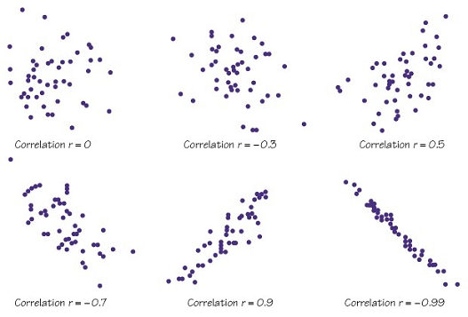
The degree of correlation between two variables is described by the coefficient of correlation r described by Pearson. It only expresses the degree of the linear relationship.
The coefficient of correlation r can vary between -1 and 1. If it is 0, then there is no correlation between the two variables – they are statistically independent.
In that case the observations would be distributed as a “hail shot” in a coordinate system.
When the coefficient of correlation increases from 0 up to 1 or decreases towards -1, the points will assemble more and more around a straight line.
When the coefficient of correlation is -1, the observations lie on a falling straight line, while if the coefficient of correlation is 1, the observations lie on a rising straight line.
Calculation of the statistical significance of the coefficient of correlation requires that the relationship between the two variables is linear and that both variables follow a normal distribution.
The requirement of linearity
In biology the relationship between two variables may not be linear. If the relationship is not linear the coefficient of correlation may be misleading.
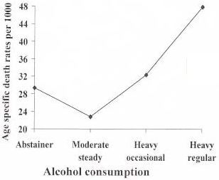
One example is that there is generally a correlation between alcohol consumption and risk of death, so that higher consumption leads to greater mortality.
At the same time it seems that a unusually modest alcohol intake is also associated with increased mortality.
There seems to be a J-shaped relationship, since mortality is highest at very modest and excessive alcohol intake and less between these extremes, corresponding to a more “normal” consumption. 
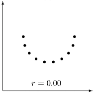
Such a relationship can, no matter how close it is, under unfortunate circumstances cause the coefficient of correlation to be 0, which can easily be misinterpreted as a sign of no association.
The coefficient of correlation is low because the association is not linear, i.e. it does not follow a straight line.
–
–
–
–
Non-parametric coefficients of correlation (Spearman and Kendall)
As an alternative to Pearson’s coefficient of correlation there are so-called non-parametric coefficients of correlation based on ranks e.g. Spearman’s rank correlation coefficient ρ (rho) and the Kendall rank correlation coefficient τ (tau).
The requirements in regard to linear relationship are less restrictive and both variables need not have a normal distribution. However, it is important to be aware that non-parametric correlation coefficients (like Pearson’s) require a monotone relation, i.e. either an ever increasing or an ever decreasing (inverse) association between variables, but they do not allow, for example, a U-shaped association.
Transformation of variables
Instead of using non-parametric methods, the requirement of linearity may often be met by suitable transformation of variables. If the side length of a cube is X, the cube’s volume V = X³. The relationship between the side length and the volume is not linear but curvilinear. If, however, a logarithmic transformation of both variables is made the coefficient of correlation will be 1 because the relationship is now linear: V = X³ ⇒ LOG (V) = LOG (X³) = 3 × LOG (X).
Compute Online
Using this link you can calculate all three coefficients of correlation i.e. Pearson’s parametric and Spearman’s and Kendall’s non-parametric coefficients of correlation.
–
–
–
–
A statistical model – Linear regression
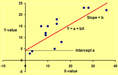
As stated above, the term relation between variables X and Y has only a statistical sense if you describe in more detail the mathematical meaning of the relationship. Such a description is called a model.  A linear relationship between the variables X and Y can be described by the following mathematical model:
Y = a + b × X
where a and b are constants (see figure). In a two-dimensional XY-plot a is the intercept of the regression line with the y-axis and b is the slope of the line (see figure). Note that X and Y are included differently in the model, Y stands alone on the left side of the equal sign, while X stands together with the constant.
Scientific hypotheses are often dealing with causal relationships, and this is reflected in the terminology. Traditionally, one imagines that X represents the cause, while Y represents the effect. Y is thus called the dependent variable (i.e., depending on X), while X is called the independent variable.
The scientific hypothesis behind the above model can be expressed as follows: Knowing the X and the constants a and b, Y can be predicted (i.e. calculated from the model).
Regression analysis
Statistically the model is analyzed using regression analysis, where one from a set of observations of paired X and Y values estimate the constants a and b and confidence intervals for the estimates. Regression analysis requires:
• linearity, i.e. a linear relationship between X and Y
• normality, i.e. that Y is normally distributed for a given X
• homoscedasticity (or variance homogeneity), i.e. the standard deviation of Y is independent of X,
• that the observations are independent.
These assumptions are best assessed visually by creating a plot of X against Y. Note that it is not a condition that X is normally distributed, and in this respect the regression analysis is different from Pearson’s coefficient of correlation (even though the calculations and the results with regard to the p-value are the same).
Compute Online
Using this link you can perform a linear regression analysis online. Here is another link which can do the same.
Many variables and multivariate statistics
Although the central issue is to illustrate the relationship between two variables X and Y, it will usually be necessary to take an interest in a wide range of other factors b1, b2, b3, etc., because they may have an influence on the interaction between X and Y).
In many projects many variables are recorded, and when the practical part of the study is completed and the data is available, the statistical task will be to analyze all the variables to get the clearest possible picture of the relationship between the variables X and Y.
Statistical analysis of many variables (X, Y, a, b1, b2, b3, etc.) is called multivariate statistics, which is complicated. The calculations are complex and cumbersome, and it was only when computers became available that the methods became more widely applied.
Before the results of a multivariate statistical analysis can be credible, a number of basic conditions must be met:
• The number of observations needs to be sufficient. Generally the reliability of statistical results increases with the number of observations. For multivariate statistics the credibility increases with the ratio between objects (individuals) and number of estimated parameters.
• As a rough rule of thumb the number of objects must be at least 10 times greater than the number of parameters.
In logistic and Cox regression analysis, the number of events (endpoints) needs to be at least 10 times greater than the number of parameters.
This means that if you plan to estimate 15 parameters in a logistic or Cox regression analysis, then there must be at least 150 events in the study. So if only 20% of the individuals develop the event, then 750 objects (individuals) need to be included in the study.
• Multivariate analysis requires a model, i.e. a basic description of the relationship between variables. The strength of the hypothetical relationship can then be assessed by the analysis, but multivariate analysis cannot operate in a vacuum without a model – in other words, if one analyzes the data on a computer using a multivariate method (e.g. multiple regression analysis), the calculations will be based on a particular model.
It is the researcher’s responsibility to ensure that the model is meaningful. It is widely accepted that the result can not be better than the data (“garbage in, garbage out”), but we often forget that the choice of an appropriate model is just as crucial to the quality of the results as the quality of the data.
• Multivariate statistics are parametric, i.e. they require that the effect variable is normally distributed. The normal distribution has a number of beautiful mathematical properties that make it possible to disentangle complex relationships between many variables. In practice, the calculations cannot be completed without the assumption of normal distribution.
We will now return to the analysis of the relationship between Y and several other variables X1, X2, X3 etc.
The responsibility of the researcher and the statistician
One often encounters the belief among scientists that if only the statistician gets all the numbers, then the statistician will analyze the relationships of the numbers and test the hypotheses that the researcher is interested in. Nothing is more wrong.
Even with a limited number of variables, the number of possible models is limitless, and therefore it is impossible with a finite set of data to determine the model. Conversely, it is crucial for the outcome of the statistical analysis, that the model is meaningful.
In practice, the model should always be determined in collaboration between researcher and statistician where the existing biological knowledge in the field (the researcher’s responsibility) is taken into account in the analysis (the statistician’s responsibility).
Known relationships should be included in the model
If for example one wishes to examine the difference in lung function between smokers and non-smokers, it is important already in the planning of the study to be aware that lung function depends on the sex, age and height. These variables should be recorded.
The relationship between lung function and sex, age and height is complex but well known from the (numerous) previous studies, and therefore it would not be appropriate from the current study limited number of observations again to analyze this context.
It is the researcher’s duty to inform the statistician about these well known relationships, and the researcher must also assist to define the model (i.e. the formulas) that should be used.
Subsequently, the statistical analysis will be both simpler and more efficient, and the statistician can concentrate on how best to describe the link between smoking and lung function, and finally – when the model is laid down in the smallest detail – to test whether this relationship is statistically significant.
–
–
–
–
Multiple regression analysis
In new research there may sometimes be little knowledge about the relationship between variables. Then one will often start with a linear model of the type:
Y = a + b1X1 + b2X2 + b3X3 + … + bnXn.
Such a model can be analyzed using multiple regression analysis, which is included in most statistical software. The model assumes simple linear relationships between the variables, which may only be partially fulfilled.
The assumptions should be checked by graphic plots of the data. Usually it is necessary to fit the model by using suitable transformations of some variables.
More complicated relationships between several variables can be described by introducing so-called interaction terms in the model. Such more complicated analyzes should be carried out in close cooperation with a qualified statistician.
More details on how to develop the model is described in the section about the Cox regression model, where the forward selection technique and the backward elimination technique are also described.
Compute Online
Using this link you can perform multiple regression analyses online.
–
–
–
–
Logistic regression analysis
As in normal regression it is a prerequisite for the statistical analysis that Y is normally distributed for a given combination of X’s. If Y is a dichotomous variable, e.g. dead / alive, this can be achieved by redefining Y.
In logistic regression analysis the dichotomous Y variable is transfomed to ln(Y / (1-Y)) (the logit) which expresses the probability of one of the two possible outcomes (for example, the probability of death for each individual).
Experience shows that the logit-transformation may be assumed to be normally distributed, but this should be checked by graphic plots of the data.
Compute Online
Using this link you can perform logistic regression analyses online.


