Welcome to The Help Page of ECstep’s Meta-Analysis Program

This page describes the facilities of the Meta-Analysis Program by ECstep and how to use it.

Data

The data you want to analyze you can 1) enter manually into the program,  2) load as an Excel file in text format, or 3) copy from Excel to the program.

1. Enter data manually into the program

You choose the menu item “Data” and then “Input or Edit Data”.

Then a new window appears, the upper part of which is shown below.

First, you should click the radio button according to the type of data you want to enter, either Binary or Quantitative. The subsequent text in the window will adapt to your choice.

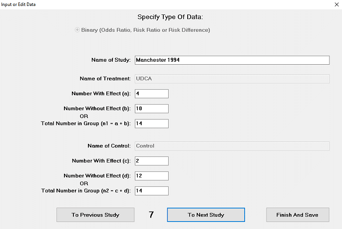
For binary data you should for each study enter the name of the study, the name of the treatment, the number with effect or response (a), the number without effect or response (b), or the total number of individuals in the group (n1 = a+b), the name of the control treatment, the number with effect or response (c), the number without effect or response (d), or the total number of individuals in that group (n2 = c+d).

When you have done this, you click “To Next Study”. Then you repeat the above steps for the next study except for the Name of Treatment and Control, which have been prefilled, since they remain the same.

If you discover a mistake, you can easily correct it as you can step through all the data by clicking “To Previous Study” or “To Next Study”.

When you have entered the data for all the studies, you click “Finish And Save”. Then you can save the data giving it a suitable name. The data will be saved in Tab-separated text format. This format can be read by Excel and other programs.

Please note that the data are entered sequentially. If you later decide to omit some studies, you should not delete them here. As described later, you can easily omit specific studies from any given analysis in a very simple way.

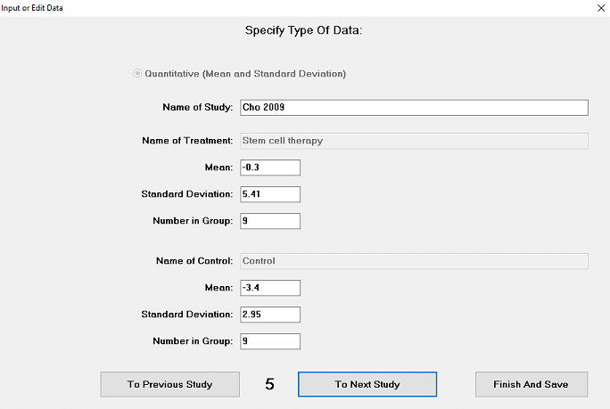
For quantitative data, you should for each study enter the name of the study, the name of the treatment, the mean, the standard deviation (SD), and the number of individuals (n1). For the control, you should enter the name of the control, the mean, the standard deviation (SD), and the number of individuals in that group (n2).

When you have done this, you click “To Next Study” as described above. Then you repeat the above steps for the next study except for the Name of Treatment and Control, which have been prefilled, since they remain the same.

If you discover a mistake, you can easily correct it as you can step through all the data by clicking “To Previous Study” or “To Next Study”.

When you have entered the data for all the studies, you click “Finish And Save”. Then you can save the data giving it a suitable name. The data will be saved in Tab-separated text format. This format can be read by Excel and other programs.

Please note that the data are entered sequentially. If you later decide to omit some studies, you should not delete them here. As described later, you can easily omit specific studies from any given analysis in a very simple way.

2. Load data in an Excel file in text format

For this to work, the data needs to be organized in nine columns in a specific order.

Binary data should be organized as shown below. The order of the nine columns as well as the header texts (line 1) should be exactly as shown.

Quantitative data should be organized as shown below. The order of the nine columns and the header texts (line 1) should be exactly as shown. Please note that the headers are different for binary and quantitative data.

For the meta-analysis program to be able to read the Excel data, it should be saved in Tab-separated text format. Excel has that facility.

3. Copy the data from Excel to the meta-analysis program

In this procedure, the data in Excel should still be organized as described above. In Excel, you select the data with all lines (including the header line) and all columns. Then you copy it, i.e. you transfer the data to the so-called clipboard. In the meta-analysis program, you click “File” and then “Import Data From Clipboard”. The program will do some data checking, and if accepted you may save it.

If Excel uses decimal commas (which is the case in some countries), the Meta-Analysis Program will automatically replace any commas with decimal points in all the numerical variables.

Before you make any analysis you may check the data in more detail. You do this by clicking “Data” and then “Input or Edit Data”. Now you can scroll through the total data set and correct any errors you may find. After that, you can save the data again and start the analysis.

Calculate

When you have the relevant data you can start the analysis. You click the menu item “Calculate” and then the specific analysis you want to perform.

Binary data

For binary data, you can choose between “Odds Ratio“, “Risk Ratio” and “Risk Difference“.

Where zeros cause problems with the computation of effects or standard errors, 0.5 is added to all cells (a, b, c, d) for that study, except when a=c=0 or b=d=0 when the odds ratio and the risk ratio are undefined. In such cases, the risk difference can still be calculated, but its standard error will tend to be underestimated by the approximate formula used.

Quantitative data

For quantitative data, you can choose between “Mean Difference” and “Standardized Mean Difference“. The latter should be used if the scale of measurement differs between the studies.

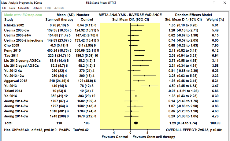
The program will calculate the specified effect measure and display the results as shown in the figure below. Each study is displayed with the name, data for the treatment and control groups, the effect measure (here the standardized mean difference) with the 95% confidence interval both graphically in the forest plot and in numbers, and the statistical weight of the study in %.

The overall effect and its significance are shown in the lower part, both graphically in the forest plot and in numbers.

The test of heterogeneity and its significance are also shown in the lower part together with I² (the percentage of the variance attributable to study heterogeneity) and tau² (an estimate of the between-study variance).

You can save the graphic results. Click menu item “File” and then “Save Graphics To file”. Then the graphic results will be saved in a bitmap file with the name you specify.

This file can be read by any graphics program including Paint and saved in JPEG format, which takes up much less space on your computer. The graphic results will be very well suited for PowerPoint presentations.

A large number of studies

The program can analyze up to 200 studies.

If you analyze a large number of studies, the results may take up more space than can be displayed fully on your computer screen at the same time. However, you can still see the total result by scrolling the various parts into view.

Furthermore, the saved graphic results file will hold the complete results. With graphic programs including Paint, you will be able to adapt and modify the total graphic results file to your specific needs.

Options

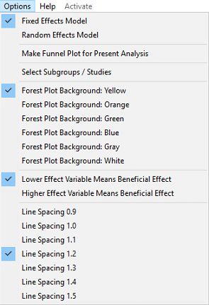
A number of options are available as shown in the menu below.

Fixed or Random Effects Model

If the heterogeneity test is not significant and I² and tau² are zero, you should be able to use the Fixed Effects Model. If on the other hand the heterogeneity test is significant and I² and tau² are not zero, you should use the Random Effects Model. However, the two model types will only give different results if tau² is above zero.

Funnel Plot

You can make a funnel plot for the present analysis. An example is shown below.

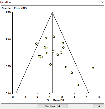
A funnel plot is a graphical tool for detecting bias in meta-analysis.

The treatment effect is plotted on the horizontal axis and the standard error (SE) on the vertical axis.

The vertical line always represents the summary effect estimated by the fixed-effect model.

The two diagonal lines represent 95% confidence limits (effect ± 1.96 SE) around the summary effect for each standard error on the vertical axis. A bias will result in an asymmetry of the funnel plot.

You can save the funnel plot by clicking “Saving Funnel Plot”. Then the plot will be saved in a bitmap file with the name you specify.

This file can be read by any graphics program including Paint and saved in JPEG format, which takes up much less space on your computer. The plot will be very well suited for PowerPoint presentations.

Select Subgroups / Studies

Sometimes it will be relevant to study subgroups to see if the results are the same in all categories. The study of subgroups will also be relevant in so-called sensitivity analyses. When you click this option the window below will appear.

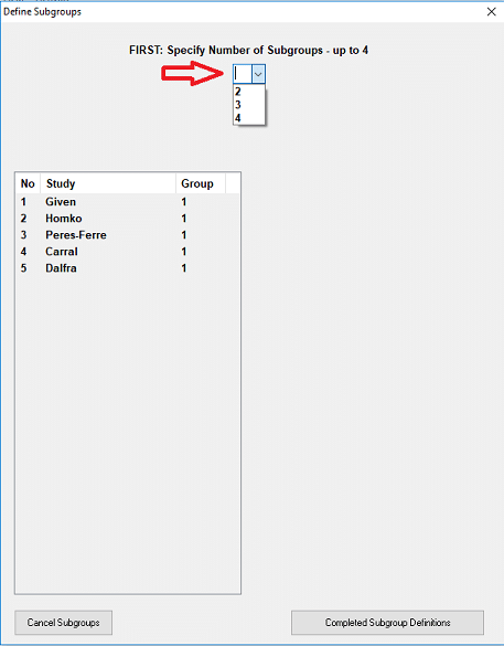
First, you define the number of subgroups. This will always have to be less than the number of studies. The program has the capacity to analyze up to nine subgroups. When you have specified the number of subgroups, the window changes to that shown below.

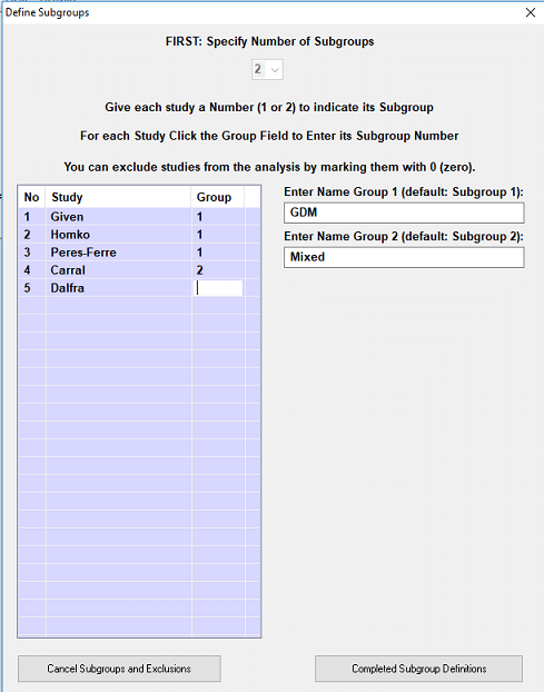
Here you can optionally give each subgroup a name. The default name will be “Subgroup x”, x being the number of the subgroup.

For each study, you click the group field to enter the number of the group the study should be in. At the start, all studies are in group 1. So you only need to enter group numbers different from 1.

Exclude studies

If you want to exclude studies from the analysis, you should enter 0 (zero) in their group field. You should not exclude any study from the data file.

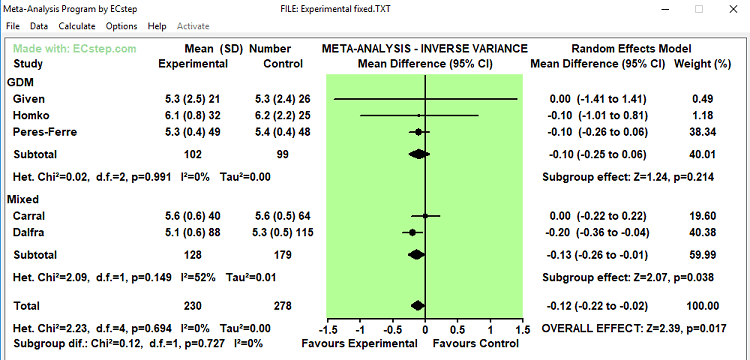
When you have finished you click “Completed Subgroup Definitions”. Then the subsequent analyses will be performed with the selected subgroups and studies. An example of subgroup analysis is shown below.

Forest Plot Background Color

You can specify the forest plot background color to be yellow, orange, green, blue, grey, or white. All subsequent analyses will be with the specified color.

Direction Of A Beneficial Effect

This option allows you to specify the direction of the beneficial effect as stated in the text directly under the forest plot. How this text should be will depend on the data being analyzed. Before you present the results you should be sure that the text is correct. The subsequent analyses will display the direction of the beneficial effect you specify.

Specify Line Spacing

The program allows you to specify the spacing between the lines in the graphic result. In some analyses with many studies, you may want to compress the results so that they can fit within a certain space (e.g. in a PowerPoint slide). The line spacings provided by the program are 0.9, 1.0, 1.1, 1.2 (default), 1.3, 1.4, and 1.5. All subsequent analyses will use the line spacing you specify.