4. Testing a hypothesis
4.86/5 (7)
Type 1 and 2 errors
A population’s precise characteristics will generally be unknown. Often, however, one will have a notion of a population’s parameters, such as the mean value of a certain variable e.g. age.
Such a concept is called a hypothesis, and the probability of the hypothesis being true can be evaluated by studying a random sample from the population.
–
–
The Hypothesis
Let’s imagine that the mean value of a particular variable in the population is M. This is our hypothesis.
We have previously seen that the distribution of means follows a t-distribution. Here we will assume the samples are large since for large samples the t-distribution will be very close to the normal distribution, which will simplify matters.
The probability of the different possible means in the samples is related to the distribution of means in samples, which is the distribution we use also for the calculation of the confidence interval.
For example, the probability that the sample mean would be outside the range M ± 1.96 x SEM would be 5%. There would be a probability of 0.025 or 2.5% of the sample mean being above the upper confidence limit, and there would be a probability of 0.025 or 2.5% of the sample mean being below the lower confidence limit.
If the mean value in a given sample falls outside the confidence interval, one would be critical as to whether the hypothesis is true, because that would only occur in 5% of cases. It would not be excluded that the hypothesis is true, but it would be less likely.
Level of significance
If you think that a 5% probability is too little to give credence to a hypothesis, you would choose to reject it if the sample mean is outside the confidence interval. You would then apply the 5% probability as the threshold value or level of significance for the decision about whether a hypothesis should be accepted or rejected.
The choice of 5% as the significance level is arbitrary but customary. However, there may well be situations where it would be justified to use a different level of significance, e.g. 10% or 1%. That would depend on the specific situation.
–
–
Significance test
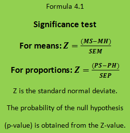
Whether a sample mean (MS) differs significantly from the hypothesis (MH) can be tested using a significance test, which calculates a test value based on the result obtained from the sample. The probability of the test value can be estimated using a known theoretical statistical distribution – in this case, the normal distribution as shown in formula 4.1.
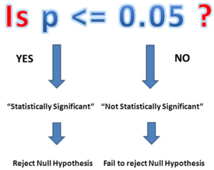
If Z is larger than 1.96 (corresponding to a probability of 2.5% in the upward direction) or smaller than -1.96 (corresponding to a probability of 2.5% in the downward direction) it is said that MS differs significantly from MH at the significance level of 5%.
Similarly, the proportion of a characteristic in a sample (PS) can be compared to the hypothetical proportion (PH) using formula 4.1 for proportions.
–
–
The p-value
The probability obtained from the significance test is called the p-value (p for probability – lower case p is used to distinguish it from the proportion P). The p-value is the probability of finding the parameter-value (and test-value) in question in a sample if the hypothesis is true.
–
–
Type 1 and type 2 errors
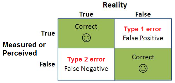
In testing a hypothesis one can commit two types of errors:
You can reject a hypothesis, even though it is true. That is a Type 1 error.
You can accept a hypothesis, even though it is false. That is a Type 2 error.
Example: The population is assumed to be audio signals from a radio. The hypothesis is that the radio is not playing music. You will commit a Type 1 error (“false positive”) if you think you hear the music, even though the radio is not playing music. You will commit a Type 2 error (“false negative”) if you cannot hear music, although the radio actually plays music.
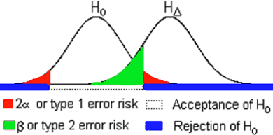
 The type 1 error probability: 2α = p-value
It follows from the definition of p-value, that the probability (risk) of a type 1 error corresponds to the p-value. This probability is also called 2α (two alpha) (the number two refers to the use of two-sided significance testing: testing for deviation in both upward and downward directions).
The type 2 error probability: β
The probability (risk) of type 2 error is indicated by β (beta). Like the choice of 2α is arbitrary (often 5%), the choice of β is also arbitrary. β is often set to 20% (10-30%).
The power: 1-β
The complementary probability 1 – β is called the power of the test. The power is the probability of rejecting a hypothesis that is false.
–
–
The null hypothesis
 Both the choice of 2α and β will depend on the relation between the hypothesis and the alternative hypotheses. For a clinical trial, the hypothesis will typically be that one therapy is better than another.
The difference between treatment effects we will call Δ (delta). The starting hypothesis is that Δ ≠ 0. All positive and negative values of Δ will fulfill the hypothesis, which makes the problem a bit confusing.
In practice, therefore one chooses to test the reverse hypothesis, i.e. that there is no difference between treatments. This hypothesis is called the null hypothesis because it assumes Δ = 0.
Then it becomes possible to test the hypothesis, but both 2α and β need to be defined as in theory there will be infinitely many alternative hypotheses, namely all positive or negative values of Δ.
In practice, the problem is solved by focusing on only one alternative hypothesis, located at a certain distance from the null hypothesis.
–
–
The minimal relevant difference
Of particular interest is the so-called minimal relevant difference Δ (effect size) between the two treatments, i.e., a difference of a certain size, which is determined when planning the study.
The type 2 error risk β will decrease (and the power 1 – β will increase) with increasing Δ and with increasing sample size.


